Introduction

Enterprises need visibility into how models are forming predictions. Mission-critical decisions cannot be made using a black box. Teams need to understand and explain how their model is making predictions. Additionally, the organization needs to understand and monitor if the model is generating unfair and partial results to certain protected classes.

ModelOp Center provides a framework for calculating, tracking, and visualizing both Model Interpretability and Ethical Fairness metrics. You can define how each of these is determined on a model by model case. You can also enforce a standard using an MLC Process as needed. The subsequent sections provide more detail on how to use ModelOp Center to implement Interpretability and Ethical Fairness into your ModelOps program.

Bias Detection

First, an example of defining the Bias Detection test. The "German Credit Data" data set classifies people described by a set of attributes as good or bad credit risks. Among the twenty attributes is gender (reported as a hybrid status_sex attribute), which is considered a protected attribute in most financial risk models. It is therefore of the utmost importance that any machine learning model aiming to assign risk levels to lessees is not biased against a particular gender.

It is important to note that simply excluding gender from the training step does not guarantee an unbiased model, as gender could be highly correlated to other unprotected attributes, such as annual income.

Open-source Python libraries developed to address the problem of Bias and Fairness in AI are available. Among these, Aequitas can be easily leveraged to calculate Bias and Fairness metrics of a particular ML model, given a labeled and scored data set, as well as a set of protected attributes. In the case of German Credit Data, ground truths are provided and predictions can be generated by, say, a logistic regression model. Scores (predictions), label values (ground truths), and protected attributes (e.g. gender) , can then be given as inputs to the Aequitas library. Aequitas's Group() calculates commonly used metrics such as false-positive rate (FPR) and false omission rate (FOR), as well as counts by group and group prevalence among the sample population. It returns group counts and group value bias metrics in a DataFrame.

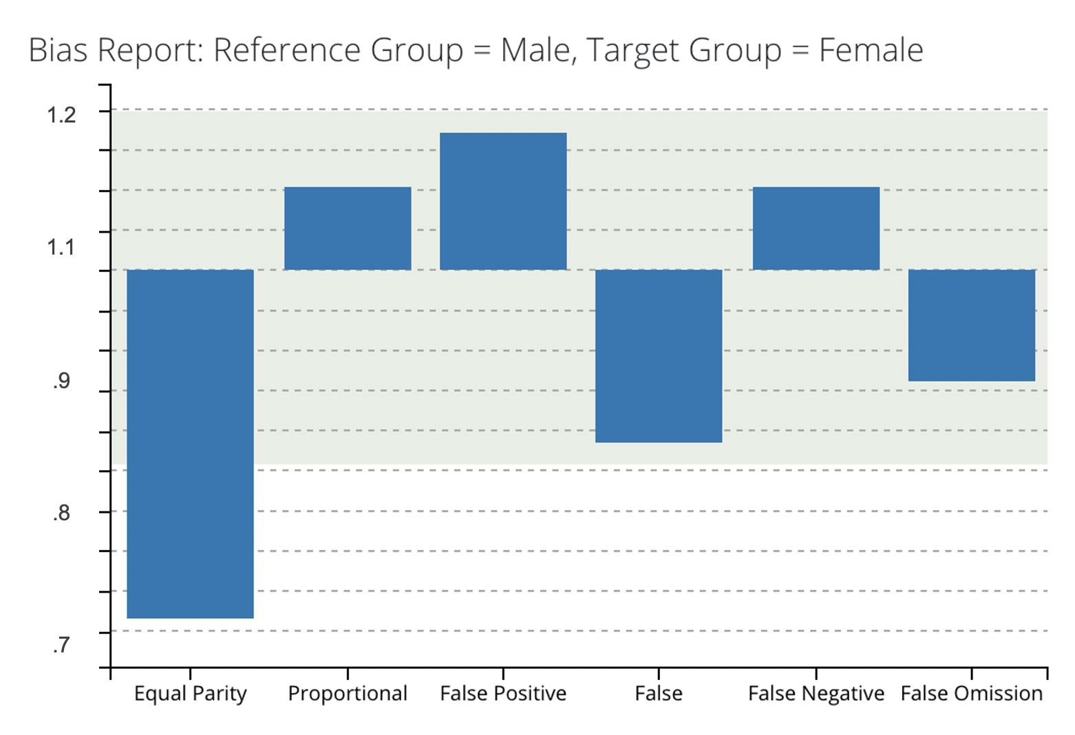
For instance, one could discover that under the trained logistic regression model, females have a FPR=32%, whereas males have an FPR=16%. This means that women are twice as likely to be falsely labeled as high-risk than as men. The Aequitas Bias() class calculates disparities between groups, where a disparity is a ratio of a metric for a group of interest compared to a base reference group. For example, the FPR-Disparity for the example above between males and females, where males are the base reference group, is equal to 32/16 = 2. Disparities are computed for each bias metric , and are returned by Aequitas in a DataFrame. This DataFrame can then be yielded by the "modelop.metrics" function, and thresholds can be set to trigger alerts for retraining when a certain model fails to meet industry standards.

Here is an example output:

Image Removed

Image Added

And here is a Metrics Function you can use to define it:

from aequitas.preprocessing import preprocess_input_df
from aequitas.group import Group
from aequitas.bias import Bias
import pickle


# modelop.metrics
def metrics(data):
    """
    Use Aequitas library to generate Group and Bias metrics
    """
    
    # Unpickle trained Logistic Regression model
    logistic_regression = pickle.load("log_reg_model.pickle")
    
    # Use model to generate predictions (scores) for input Dataset
    data_scored = data.copy(deep=True)
    data_scored["score"] = logistic_regression.predict(data)
    
    # To measure Bias towards gender, filter DataFrame
    # to "score", "label_value" 
    # (ground truth), and
    # "gender" (protected attribute)
    
    data_scored = data_scored[
        ["score", "label_value", "gender"]
    ]
    
    # Process DataFrame
    data_scored_processed, _ = preprocess_input_df(data_scored)
    
    # Group Metrics
    g = Group()
    xtab, _ = g.get_crosstabs(data_scored_processed)
    
    # Absolute metrics, such as 'tpr', 'tnr','precision', etc.
    absolute_metrics = g.list_absolute_metrics(xtab)
    
    # DataFrame of calculated absolute metrics for each sample population group
    absolute_metrics_df = xtab[
        ['attribute_name', 'attribute_value'] + absolute_metrics].round(2)
        
    # For example:
    """
        attribute_name  attribute_value     tpr     tnr  ... precision
    0   gender          female              0.60    0.88 ... 0.75
    1   gender          male                0.49    0.90 ... 0.64
    """
    
    # Bias Metrics
    b = Bias()
    
    # Disparities calculated in relation gender for "male" and "female"
    bias_df = b.get_disparity_predefined_groups(
        xtab,
        original_df=data_scored_processed,
        ref_groups_dict={'gender': 'male'},
        alpha=0.05, mask_significance=True
    )
    
    # Disparity metrics added to bias DataFrame
    calculated_disparities = b.list_disparities(bias_df)
    
    disparity_metrics_df = bias_df[
        ['attribute_name', 'attribute_value'] + calculated_disparities]
        
    # For example:
    """
        attribute_name	attribute_value    ppr_disparity   precision_disparity
    0   gender          female             0.714286        1.41791
    1   gender          male               1.000000        1.000000
    """
    
    output_metrics_df = disparity_metrics_df  # or absolute_metrics_df
    
    # Output a JSON object of calculated metrics
    yield output_metrics_df.to_dict()
    

Interpretability

While model interpretability is a complex and rapidly-changing subject, especially for AI models, ModelOp Center can assist you in understanding and calculating how much each feature contributes to the output of each individual prediction. In other words, these metrics show the impact of each feature on each prediction. ModelOp Center does this by leveraging SHAP to automatically compute the feature importance metrics. The SHAP results are persisted with the Test Results for the model for auditability. Note: not all models are easily interpretable, and as a result, model interpretability can be used as a factor for deciding the approach and choice of a model.

The following example uses the SHAP library to calculate the impact of the features on the prediction. It emits the average SHAP value for each feature and yields it as a dictionary.

# modelop.metrics
def metrics(data):
    standard_data = data
	shap_values = []
	
    for standard_datum, datum in zip(standard_data, data)
		for k in means.keys():
        	standard_datum[k] = (datum[k] - means[k]) / stdevs[k]
    	if not datum['GarageYrBlt']:
        	datum['GarageYrBlt'] = garageyrbuilt_mean
    	idx = standard_datum.pop("Id")
    	pd_datum = pd.DataFrame(standard_datum, index=[idx], columns = features)
    	shap_values.append(shap_explainer.shap_values(pd_datum.values)[0])
	
	shap_values = pd.DataFrame(shap_values, names=features)
	shap_means = shap_values.apply(numpy.abs, axis=1).mean()
	
    yield shap_means.to_dict.()

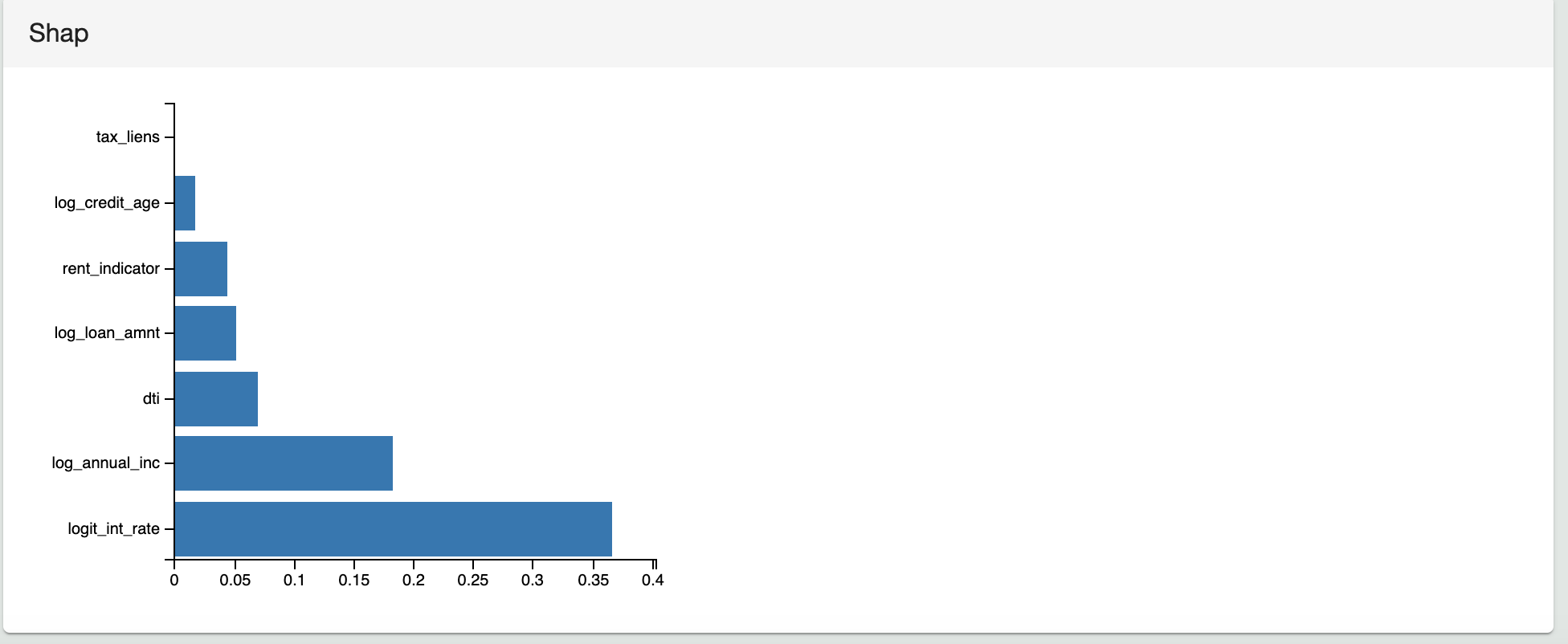
The following image shows the corresponding visualization for the shap SHAP values of the sample model to the Test Results in ModelOp Center.

Next Article: Model Governance: Model Versioning >