Introduction

Enterprises need visibility into how models are making predictions. Mission-critical decisions cannot be made using a black box. Teams need to understand and explain model outputs. One such method is by understanding how each of the input features is impacting the outcome.

ModelOp Center provides a framework for calculating, tracking, and visualizing Model Interpretability metrics. Each of these can be determined on a model-by-model basis. You can also enforce a standard using an MLC Process as needed. The subsequent sections provide more detail on how to use ModelOp Center to implement Interpretability into your ModelOps program.

Interpretability in MOC

While model interpretability is a complex and rapidly-changing subject, ModelOp Center can assist you in understanding how much each feature contributes to the prediction, as well as monitoring each feature’s contribution over time. ModelOp Center does this by expecting a trained SHAP explainer artifact and finding the SHAP values over the input dataset. The SHAP results are persisted for auditability and tracking over time.

The following example uses the SHAP library to calculate the impact of the features on the prediction, calculates the average SHAP value for each feature, then returns it as a dictionary.

Code Block

language	py

import pandas as pd
import numpy as np
import shap
import pickle
from scipy.special import logit


# modelop.init
def begin():
    
    # Load SHAP explainer, model binary, and other parameters into global variables
    global explainer, lr_model, threshold, features

    model_artifacts = pickle.load(open("model_artifacts.pkl", "rb"))
    explainer = model_artifacts['explainer']
    lr_model = model_artifacts['lr_model']
    threshold = model_artifacts['threshold']
    features = model_artifacts['features']

    pass


def preprocess(data):
    """
    A Function to pre-process input data in preparation for scoring.
    
    Args:
      data (pandas.DataFrame): Input data.
    Returns:
      (pandas.DataFrame): Prepped data.
    """
    
    prep_data = pd.DataFrame(index=data.index)
    prep_data["logit_int_rate"] = data.int_rate.apply(logit)
    prep_data["log_annual_inc"] = data.annual_inc.apply(np.log)
    prep_data["log_credit_age"] = data.credit_age.apply(np.log)
    prep_data["log_loan_amnt"] = data.loan_amnt.apply(np.log)
    prep_data["rent_indicator"] = data.home_ownership.isin(['RENT']).astype(int)

    return prep_data


def prediction(data):
    """
    A function to predict on prepped input data, using the loaded model binary.
    """
    return lr_model.predict_proba(data.loc[:, features])[:,1]


def get_shap_values(data):
    """
    A function to compute and return sorted SHAP values, given the loaded SHAP explainer.
    """
    
    shap_values = explainer.shap_values(data.loc[:, features])
    shap_values = np.mean(abs(shap_values), axis=0).tolist()
    shap_values = dict(zip(features, shap_values))
    sorted_shap_values = {
        k: v for k, v in sorted(shap_values.items(), key=lambda x: x[1])
    }
    return sorted_shap_values

# modelop.metrics
def metrics(data):

    metrics = {}
    # Prep input data
    prep_data = preprocess(data)
    data = pd.concat([data, prep_data], axis=1)
    
    # Compute predictions
    data.loc[:, 'probabilities'] = prediction(data)
    data.loc[:, 'predictions'] = data.probabilities \
                                     .apply(lambda x: threshold > x) \
                                     .astype(int)
    # Compute SHAP values
    metrics['shap'] = get_shap_values(data)

    return metrics

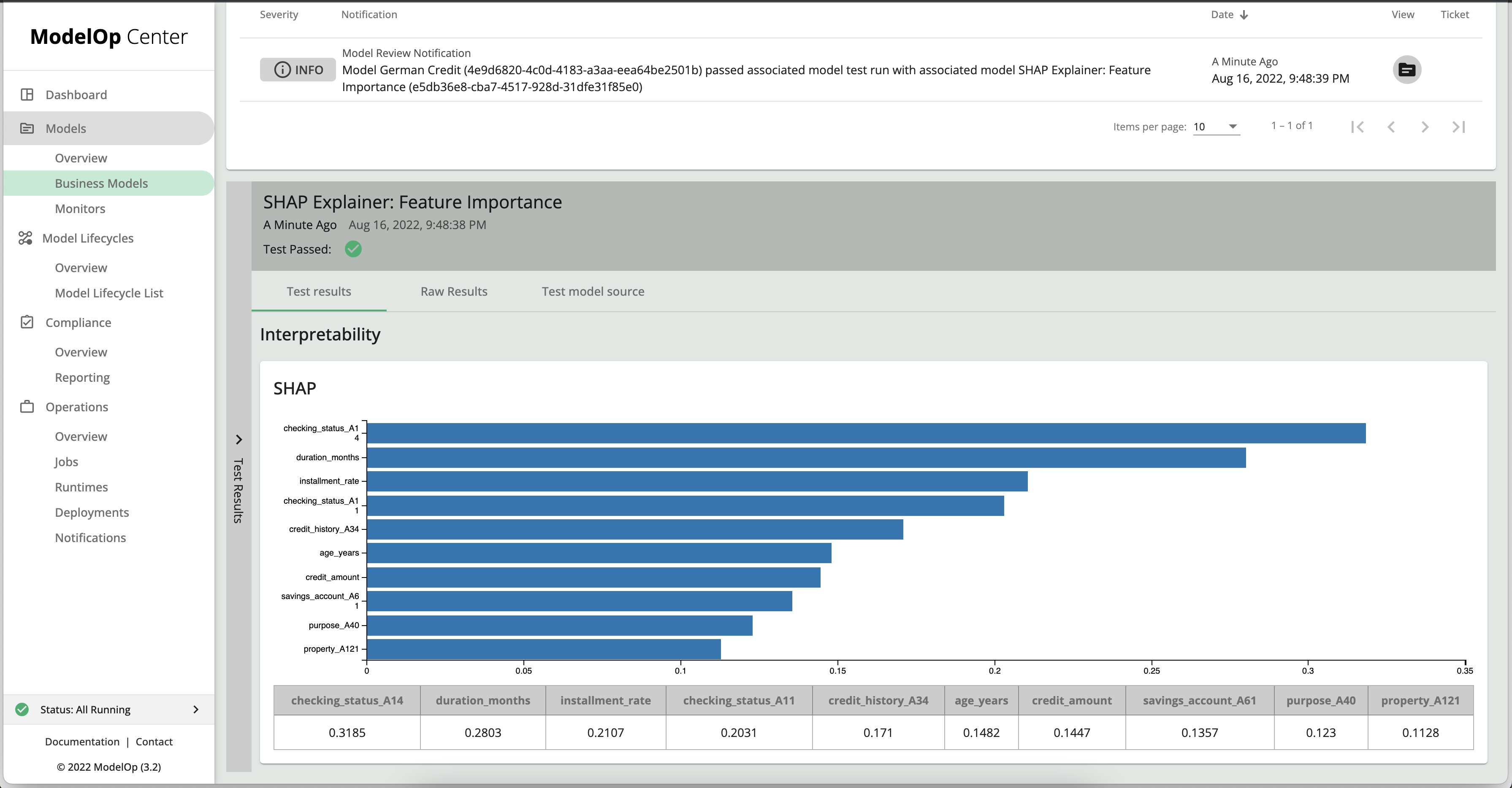
The following image shows the corresponding visualization for the SHAP values of the sample model to the Test Results in ModelOp Center.

Image Removed

In the sections below we will demonstrate how an explainability monitor can be setup in MOC. The example used is based on the German Credit business model, which can be found here. The business model is the base model producing inferences (predictions). The SHAP monitor can be found here. The monitor is itself a storedModel in MOC.

Adding a SHAP monitor to a business model

To add the SHAP monitor referenced above to the German Credit (GC) model, follow these steps:

Import the GC model into MOC by Git reference.
Create a snapshot of the GC model. In doing so, it is not necessary to deploy the snapshot to any specific runtime, as we will not be running any code from the GC model itself.
Import the Feature Importance monitor by Git reference.
Create a snapshot of the monitor. You may specify a target runtime on which you’d like the monitoring job to be run.
Associating the monitor to the business model:
1. Navigate to the GC model spapshot,a nd click on ADD, then on MONITOR.
  Image Added
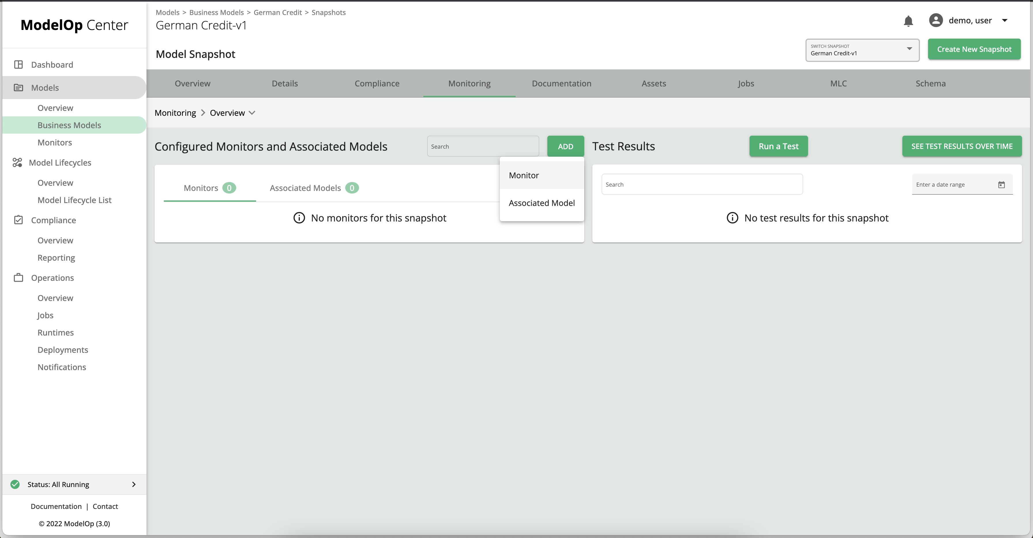
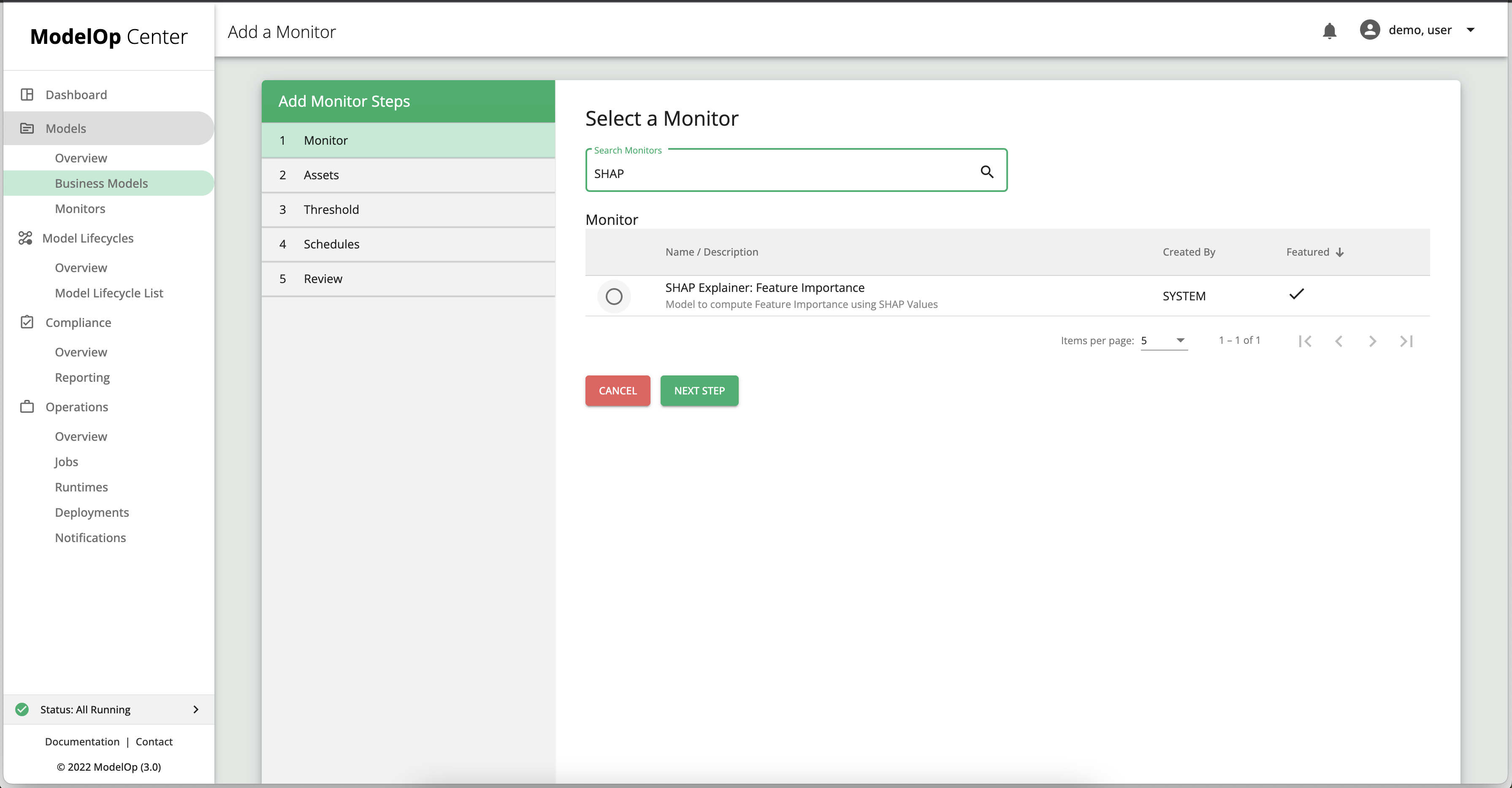
2. Select the SHAP monitor from the list of monitors, and then select its snapshot.
  Image Added
3. On the Assets page:
  1. Select an input asset from the existing data assets of the GC business model, say, df_sample_scored.json. In a PROD environemnt, you are more likely to add a SQL asset (by connection and query string), or an S3 asset (by URL).
  2. under “Additional Assets”, select the existing assets shap_explainer.pickle for Pre-trained SHAP explainer, and predictive_features.pickle for List of predictive features as used by scoring model.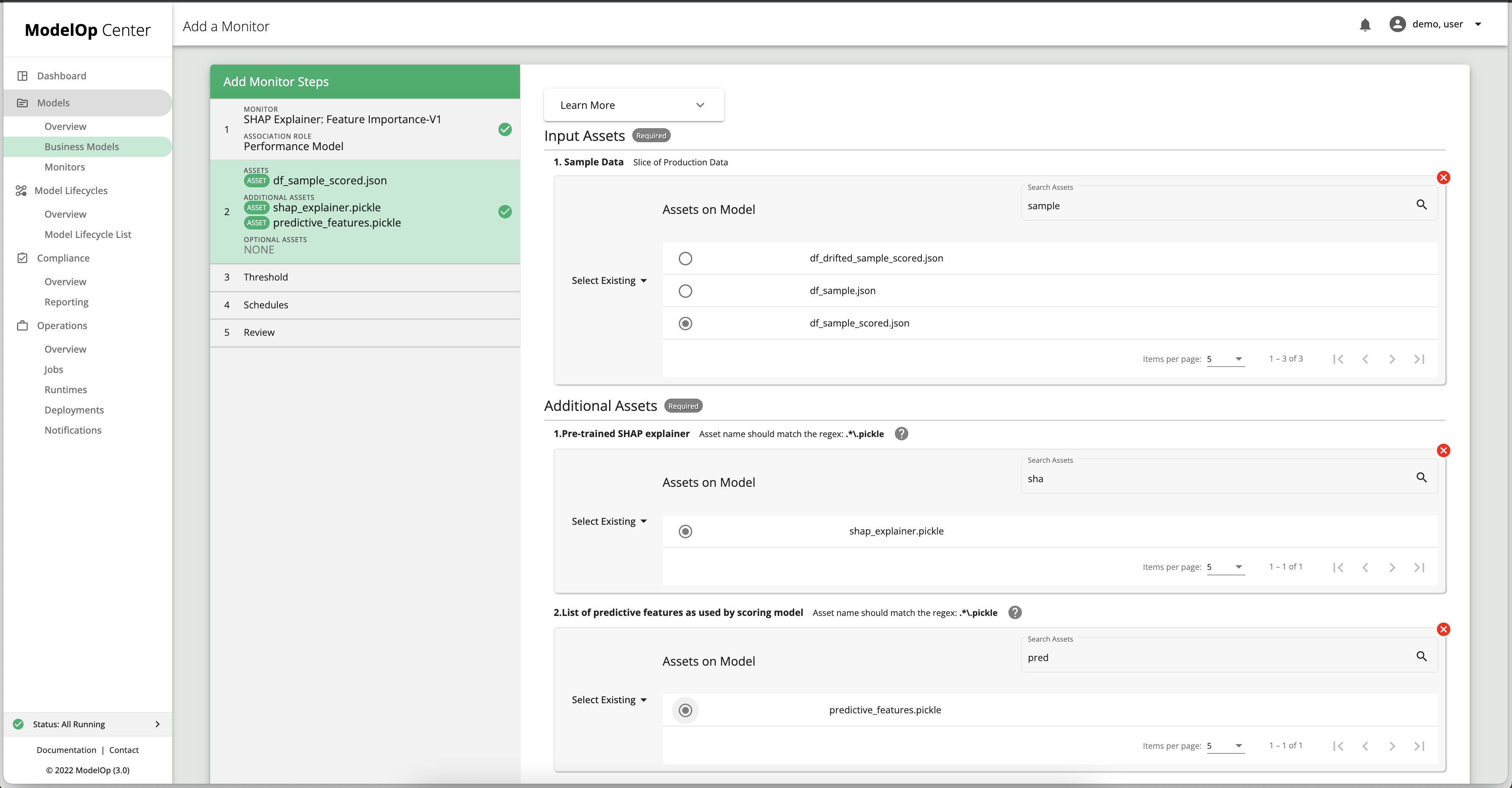
    Image Added
  3. Click Next.
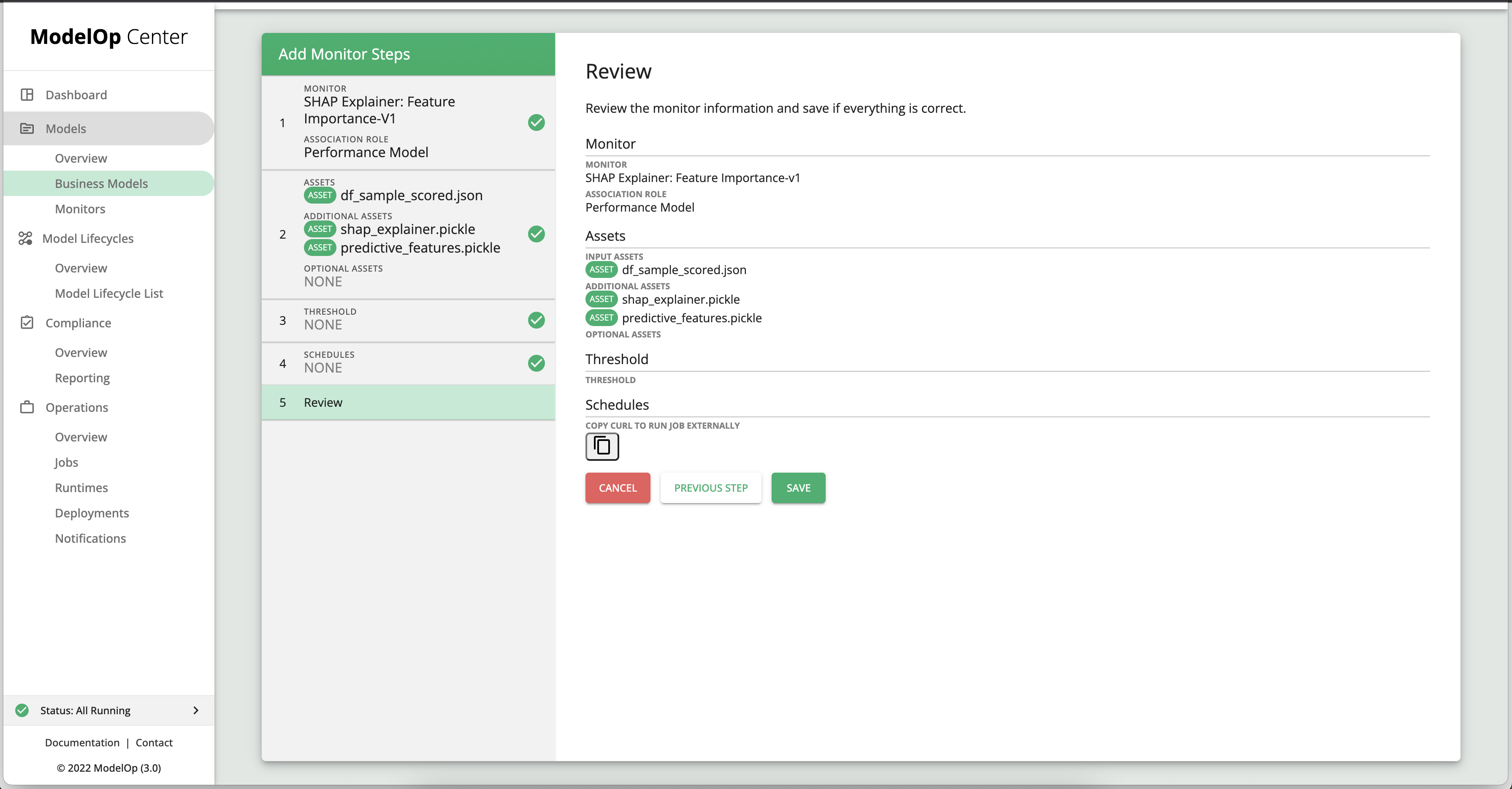
4. For this example we will skip the Threshold and Schedule steps.
5. On the last page, click Save.
  Image Added
To run the monitor, navigate to the snapshot of the GC model, and then to monitoring.
Under the list of monitors, click the play button next to the SHAP monitor to start a monitoring job. You will then be re-directed to the Jobs page, where you’ll be able to look at live logs from the monitoring run.
Image Added
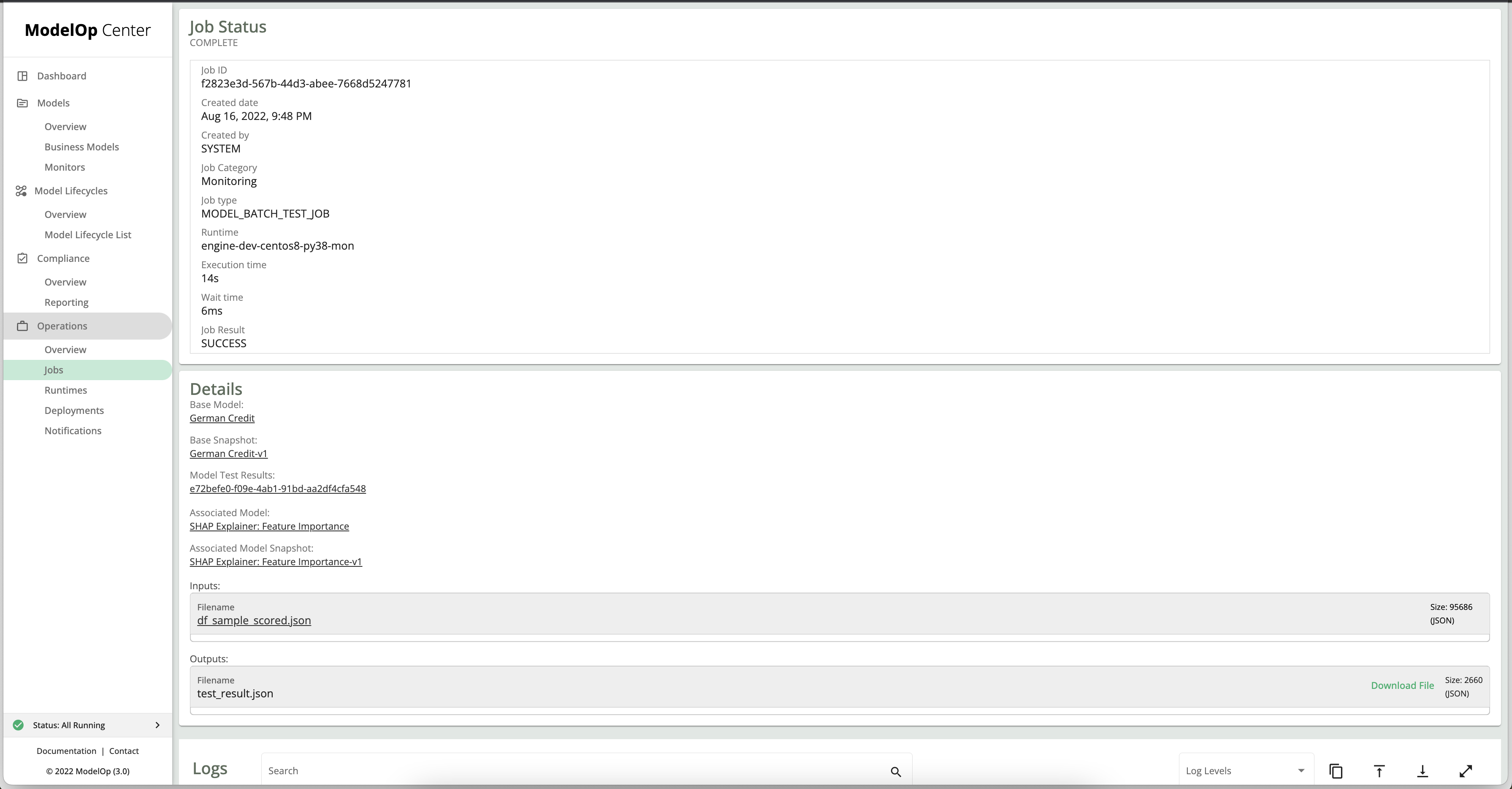
To download the Test results, click on Download File in the Details box. To view a graphical representation of the test result, click on the Model Test results UUID link in the Details box. You will be re-directed to the snapshot’s monitoring page, and presented with the following output:
Image Added